
knowledge-graph-rdbms
<!-- mcp-name: io.github.cunicopia-dev/knowledge-graph-rdbms -->






An embedded knowledge graph you own completely — in one SQLite file.
SQLite-native · zero-dependency core · MCP-ready · event-sourced · reversible.
Model anything as entities and relationships — agent memory, app ontologies, declarative datasets, "SQLite but my data is a graph" — without running Neo4j, RDF, Docker, or a separate graph service. No Cypher, no JVM, no server: five tables and one file you can copy, inspect, and version.
pip install "knowledge-graph-rdbms[mcp]"

# write a fact — auto-creates the graph in one SQLite file
kg node add person:ada --kind Person --name "Ada Lovelace"

# every write is logged; tail the log and roll any event back by id
kg events -n 5
kg revert <event_id>

# rebuild the graph as of any past moment — literal time travel
kg replay --upto 2026-01-01T00:00:00

# expose the whole graph to an AI agent over MCP
kg serve
   Agent / CLI / Python
            │
     gated + logged writes
            │
   SQLite label property graph
            │
    replay · revert · time-travel
Python 3.10+ · MIT · zero-dependency core · library + CLI + MCP
The world isn't rows in a table — it's things, the kinds of things they are, and how they relate. A label property graph captures exactly that, and not much more: nodes (entities), typed edges (relationships), labels (sets), and JSON properties (everything else). There's no schema to design up front; meaning accretes as facts, and the shape stays as flexible as the domain it describes.
That flexibility is what makes it a natural substrate for AI agents. Hand an agent an MCP connection to this graph and it can do what agents are uniquely good at: read a domain, model what it learns, connect ideas, and reason over structure instead of prose. Every write is gated, attributed, and appended to an event log — so an agent can reshape the graph freely while you keep the receipts: audit it, replay it to any point in time, or roll a change back with one command. A memory that records why, not just what — in one embeddable file that travels wherever the agent runs: a laptop, a CI job, a serverless function, a Pi.
Small enough to hold in your head. Flexible enough to model anything.
Contents
- Where it fits
- Why not X?
- The idea in 30 seconds
- Design philosophy
- The data model
- Architecture: three front doors, one engine
- Many ontologies: one control plane
- Discovery: read the schema before you query
- Cross-ontology: federation and the backbone
- Event sourcing: the graph is a projection
- The safety gate: invariants vs. policy
- Install
- Quickstart
- Performance
- RDF interop: export, SPARQL, RDF-star
- Command reference
- Project layout
- Development
- License
Where it fits
It's built for graphs you want to own completely — small enough to inspect, fast enough to embed, transparent enough to trust:
- Embedded ontologies — a knowledge graph that ships inside a single app or service, in one file you can copy and version.
- Agent & assistant memory — facts an AI can read and write over MCP, with a full audit trail and one-command rollback.
- Declarative datasets — describe your base graph as YAML/JSON facts and replay them into a queryable graph, deterministically.
- "SQLite, but my data is a graph" — the moment relational rows start describing relationships, this is their natural home.
The design center is read-heavy, single-writer, up to low millions of nodes — the same sweet spot as SQLite itself: one file, in-process, no server to run. That covers a surprising amount of real work. For workloads past that center, Performance maps out exactly where the curve bends and a purpose-built graph engine starts to earn its extra moving parts.
Why not X?
Honest comparisons — reach for the right tool, and know exactly when that tool is this one.
Why not Neo4j?
Use Neo4j when you need deep traversal, complex Cypher pattern matching, concurrent writers, or clustered graph infrastructure. Use kgrdbms when you want a small embedded graph, agent memory, auditability, local-first ownership, and SQLite deployment simplicity.
Why not NetworkX?
NetworkX is great for in-memory algorithms. kgrdbms is for persistent graph state with durable storage, CLI/MCP access, event history, and rollback.
Why not RDFLib?
RDFLib is for RDF graphs and linked-data workflows. kgrdbms is a label property graph with RDF as an export/import boundary, not a triplestore.
Why not just SQLite tables?
Because some domains are naturally entities and relationships, not rectangular tables. kgrdbms keeps the storage boring while making the model graph-shaped.
The idea in 30 seconds
A label property graph needs only four primitives:
| Primitive | What it is |
|---|---|
| Node | a stable id, a kind, a display name |
| Edge | a typed, directed relationship between two nodes |
| Label | set memberships on a node (many per node) |
| Property | a JSON-valued key/value bag on a node or an edge |
Store those in SQLite, add a few indexes, and you have a knowledge graph. Everything else in this project — traversal, an append-only history, a safety gate, the CLI, the MCP server — is built on top of those four facts.
from kgrdbms import Graph

with Graph(path="demo.db") as g:
    g.add_node("person:ada", kind="Person", name="Ada Lovelace",
               labels={"Person"}, properties={"born": 1815})
    g.add_node("field:cs", kind="Field", name="Computer Science")
    g.add_edge("person:ada", "field:cs", "FOUNDED", properties={"year": 1843})

    print(g.shortest_path("person:ada", "field:cs"))
flowchart LR
    ada(["person:ada<br/>:Person<br/>born=1815"])
    cs(["field:cs<br/>:Field"])
    ada -->|"FOUNDED (year=1843)"| cs
Design philosophy
1. Boring storage is a feature. SQLite already solved durability, transactions, indexes, and recursive queries. We don't reinvent any of it. One file, copy it to back it up, open it with any SQLite tool to inspect it.
2. The schema fits on a screen. Five tables, no surprises. You can read the entire storage layer and know exactly where every fact lives. Legibility beats cleverness.
3. The state is a pure function of data. What you query is a projection.
The source of truth is an append-only log of facts plus an optional declared
seed. Your whole graph is reproducible: state = replay(seed + log). That one
property buys audit, undo, and time-travel for free.
4. Mutation is gated, and the gate has two layers. When you let an agent rewrite your graph over a wire, you need rules. Some rules are configurable (policy); some must be un-negotiable (compiled-in invariants). We separate mechanism from policy on purpose.
5. One engine, many doors. A library call, a kg command, and an MCP tool
all flow through the same gated, logged write path into the same file. There is
no "CLI version" of the truth and "MCP version" of the truth — there's one.
6. Pay for speed only when you ask. Every single write commits on its own
(safe by default). Bulk paths (batch(), add_nodes, add_edges) let you opt
into ~10× throughput when you mean to.
The data model
The graph is five tables. That's the whole storage layer.
erDiagram
    nodes ||--o{ node_labels : "is labeled"
    nodes ||--o{ node_properties : "has"
    nodes ||--o{ edges : "from / to"
    edges ||--o{ edge_properties : "has"

    nodes {
        text id PK
        text kind
        text name
        text created_at
    }
    node_labels {
        text node_id FK
        text label
    }
    node_properties {
        text node_id FK
        text key
        text value_json
    }
    edges {
        text id PK
        text from_node FK
        text to_node FK
        text type
    }
    edge_properties {
        text edge_id FK
        text key
        text value_json
    }
Design notes that matter:
- Edges are unique on
(from_node, type, to_node). Re-adding the same triple updates its properties instead of duplicating it. Idempotent by construction. - Properties are JSON. Values round-trip as whatever JSON type you store — ints, bools, lists, nested objects.
- Foreign keys cascade. Delete a node and its labels, properties, and incident edges go with it, enforced by SQLite.
slug()deduplicates natural-language ids. Two strings that slugify the same become the same node — the load-bearing trick for turning prose concepts into stable ids.- Ids are CURIEs.
person:ada-lovelace,company:apple— a compact URI:prefix:reference, where the prefix is a short stable type token and the reference is slugged (slug(name, prefix="person")mints them). It stays a plain string today and expands to a full IRI only the day you publish to the linked-data world, so interop is a cheap, additive option rather than a tax paid up front. The id is an address, not a record: identity goes in the id, changeable facts go in properties.
A sixth table, graph_events, holds the append-only history (see below). It
shares the same file and connection.
Architecture: three front doors, one engine
flowchart TD
    subgraph doors["front doors"]
        CLI["kg<br/>(command line)"]
        MCP["kgrdbms-mcp<br/>(MCP server)"]
        LIB["import kgrdbms<br/>(library)"]
    end

    SVC["service.py — gated + logged write path"]
    GATE{"invariants.enforce<br/>then policy.mutation_check"}
    GRAPH[("SQLite file<br/>nodes · edges · labels · properties")]
    LOG[["graph_events<br/>(append-only log)"]]

    CLI -->|writes| SVC
    MCP -->|writes| SVC
    LIB -->|writes| SVC
    SVC --> GATE
    GATE -->|"pass"| GRAPH
    GATE -->|"record fact"| LOG

    CLI -.->|reads| GRAPH
    MCP -.->|reads| GRAPH
    LIB -.->|reads / fast bulk writes| GRAPH
The CLI, the MCP server, and your own Python code all mutate through
service.py, so the safety gate and the event-log bookkeeping exist in exactly
one place and can't drift between front doors.
The gate resolves invariants.enforce and policy.mutation_check through
their modules at call time — so editing your policy (or monkeypatching it in a
test) takes effect across every door at once.
The library also has a direct, fast, unlogged path (
g.add_node(...),g.add_nodes(...)). It's the right tool for bulk loading, but those writes are not in the event log — see the warning under Event sourcing.
Many ontologies: one control plane
One graph is the engine. The control plane lets all three front doors
address many named ontologies through that one engine — each its own SQLite
file (and, when a workload earns it, its own engine entirely). You name an
ontology; the resolver routes. Nothing else changes — the gate, the log, and the
service.py write path are exactly the same; only which graph + log they act
on is chosen by name.
flowchart TD
    subgraph doors["front doors, now ontology-aware"]
        CLI["kg --ontology coffee …"]
        MCP["kg_node_get(ontology='coffee')"]
        LIB["resolve('coffee')"]
    end
    RES["resolver.py<br/>name → (backend, events, entry)"]
    IDX[["index.db<br/>the registry — itself a kg"]]
    REG{"backend registry"}
    SQ[("sqlite · live")]
    PG[("postgres · live")]
    NEO[("neo4j · stub")]

    CLI --> RES
    MCP --> RES
    LIB --> RES
    RES -->|"look up the name"| IDX
    RES -->|"open the engine"| REG
    REG --> SQ
    REG -.-> PG
    REG -.-> NEO
- The registry is itself a kg. Ontologies are nodes in an index graph
(
<root>/index.db), so listing them is a query and registering one is an upsert — no new storage machinery. A database of databases. - The default ontology is the legacy file. Omit the name and you hit
<root>/graph.db, exactly as before. Multi-ontology is purely additive; nothing moves, and every existing command behaves identically. - Isolation is filesystem-shaped. Each ontology is its own file with its own event log. "Coffee doesn't know Ada" because they are different files — no tenant ids, no row filtering, no leak surface.
- The engine is pluggable. A backend is a factory registered under a name.
sqliteandpostgresare live;neo4jis a stub that routes and fails loudly until built. Most ontologies stay embedded SQLite — the zero-dependency default — while a specific heavy one can be escalated to a purpose-built engine when its workload (not its row count) turns deep. Philosophy #6, "pay for speed only when you ask," generalized from batching to whole engines. - History is owned by the control plane, not the engine. A non-sqlite
ontology keeps its append-only event log in a control-plane SQLite store
(
<root>/ontologies/<slug>/events.db); the engine is just the projection that replay and undo apply to. So a Postgres-backed ontology still gets the full audit / time-travel / one-command-revert story — graph data in Postgres, history in SQLite.
pip install "knowledge-graph-rdbms[postgres]"     # the psycopg-backed engine
kg ontology create big --backend postgres \
   --location "postgresql://user:pass@host:5432/db" --stance inferential
kg --ontology big node add company:acme --kind Company --name Acme   # writes to Postgres
kg ontology create coffee --stance inferential       # register (lands in index.db)
kg ontology list                                     # the database of databases
kg --ontology coffee node add drink:latte --kind Drink --name Latte
kg --ontology coffee out drink:latte                 # scoped to that ontology
Two ways to target a graph, mirroring the MCP ontology argument: --ontology NAME routes through the resolver (named, registered, multi-engine), while
--db PATH stays the raw escape hatch onto one exact file, registry untouched.
Discovery: read the schema before you query
A graph you didn't build is opaque: which kinds exist? which edge types? what
property keys live on a Person? schema() answers all of it in one read —
the map to read before querying, rather than guessing with trial calls.
kg schema             # kinds, edge types, labels, and property keys per kind — with counts
kg schema --samples   # + a few example ids per kind and the enum-like values a key takes
What comes back is the observed vocabulary — a profile of what's actually in
the graph, not an enforced schema (the graph stays schemaless). The MCP tool
kg_schema carries an instruction to call it first, so an agent reads the map
before it moves. It's a plain read — pure GROUP BY aggregates, no gate — and
like every read it has a federated form (next) that unions the vocabulary across
many ontologies at once.
Cross-ontology: federation and the backbone
The control plane routes to one ontology per call. Two layers sit on top to work across many at once: reads federate, writes go through a backbone.
flowchart TD
    Q["kg fed node person:ada"] --> FED["federation.py<br/>multithreaded fan-out"]
    FED -.->|own thread + connection| O1[("people")]
    FED -.->|own thread + connection| O2[("papers")]
    FED -.->|own thread + connection| O3[("coffee")]
    O1 --> M["merge, tagged by source<br/>(identity-aware)"]
    O2 --> M
    O3 --> M

    L["kg link same-as …"] --> BB["backbone.py"]
    BB --> IDX[["index.db — the backbone<br/>Ref + Prefix nodes, SAME_AS edges<br/>gated + logged"]]
Federation — cross-ontology reads, multithreaded
A federated read is a fan-out: open each member ontology in its own thread (its
own connection — SQLite releases the GIL during a query, so N ontologies read
concurrently) and merge the results tagged by source. There's no separate
"federated" API: every base read takes an optional ontologies=[...] scope.
from kgrdbms import Federation

fed = Federation(["people", "papers", "coffee"])   # or Federation.all()
fed.schema()                 # unioned vocabulary + a per-ontology breakdown
fed.nodes_by_kind("Person")  # [Located(ontology, node), ...] — tagged by source
fed.node("person:ada")       # every occurrence across worlds, identity-merged
kg fed schema                # union vocabulary across ALL ontologies
kg fed node person:ada       # find an id across the federation (identity-aware)
Federation never writes and never silently drops a member (a member that raises
propagates); parallel=False forces sequential for debugging.
The backbone — cross-ontology links
A leaf edge can't cross ontologies: its foreign key lives in one file. The backbone
is where cross-ontology structure lives, and it needs no new storage — it is the
index graph growing new kinds. A link becomes a lightweight Ref proxy node per
endpoint (id <ontology>::<node_id>, FK-satisfied inside the index) joined by an
edge; the prefix registry becomes Prefix nodes. Both go through the same gated +
logged service path, so a cross-domain assertion is audited, reversible, and
replayable exactly like leaf data.
kg link add coffee drink:latte ENJOYED_BY people person:ada   # a typed cross-ontology edge
kg link same-as people person:ada wiki person:ada-lovelace    # "same real-world entity" (symmetric)
kg link cluster people person:ada                             # the transitive SAME_AS cluster
kg prefix add person https://kg.local/person/                 # CURIE prefix -> IRI (identity backbone)
Identity is opt-in per ontology. By default identity is local — person:ada
in two ontologies are different nodes until you link them via the backbone. An
ontology created with --shared-identity opts into global identity, and federation
then treats same-CURIE nodes across such ontologies as the same entity and merges
them.
Event sourcing: the graph is a projection
The graph you query is a cache. The append-only event log is the source of truth. Every gated mutation records a reversible fact.
flowchart LR
    SEED["genesis seed<br/>(optional, declarative)"] -->|"seed once"| PROJ
    LOG[["event log<br/>append-only, never deletes a row"]] -->|"replay in order"| PROJ[("graph projection<br/>what you query")]
    PROJ -->|"every gated mutation appends a fact"| LOG
Because the log never loses a row, you get three things at once:
- Audit is archaeology. Every change is timestamped and attributed to an
actor.
kg eventstails the history. - Undo is an event, not a delete.
compensate()(CLI:kg revert <id>) emits the inverse event. The original row stays; you can see that it was reverted and by what. - Time travel.
replay(upto_ts=...)rebuilds the projection as of any past instant.
sequenceDiagram
    participant U as you
    participant L as event log
    participant G as graph projection
    U->>L: NODE_UPSERT person:ada
    L->>G: apply → ada exists
    U->>L: revert(that event)
    L->>L: append NODE_DELETE (compensates)
    L->>G: apply → ada gone
    Note over L: both rows remain — history is intact
Two write paths, by design
You choose how each write relates to history:
- Logged path — the CLI, the MCP server, and
service.*. Every mutation is gated and appended to the log, so it's audited, reversible, and reproduced exactly byreplay(). This is the path you want when the timeline is the truth. - Direct path —
g.add_node,g.add_nodes,g.batch(). Writes go straight to the projection: the fastest way to bulk-load or stage data. They aren't in the log, soreplay()(which rebuilds from the log) won't include them.
Pick per workload: direct for raw loading speed, logged when you need the
history. And you can have both — kg import runs the logged path inside a
single batch(), so a bulk load is fast and fully recorded.
The replay seed is just a callable, so you can declare your base graph in YAML/JSON and re-seed deterministically before the logged deltas are applied:
from kgrdbms import Graph, EventLog, replay

def genesis(g):
    # re-create your declared base facts (e.g. parsed from YAML)
    g.add_node("root", kind="Root", name="root")

replay(graph, events, genesis=genesis)              # rebuild from seed + log
replay(graph, events, genesis=genesis, upto_ts=ts)  # ...as of an instant
Virtual edges: relationships you don't store
Event sourcing is the right model for curated facts — but the wrong one for a high-cardinality, machine-generated relationship layer that already lives, fresh and authoritative, in some operational store. Mirroring 100k correlation edges into the graph (and the log) every night is wasteful and instantly stale.
A virtual edge inverts that. The ontology stores only a binding — an edge TYPE plus the SQL that resolves its instances against an external source. At traversal time the resolver runs that query, parameterized by the node you're standing on, and synthesizes the edges live. Zero copy, always current, one source of truth — Ontology-Based Data Access in the graph's own terms.
flowchart LR
    Q(["kg_edges('company:NVDA')"]) --> U{"union traversal"}
    STORE[("event-sourced graph<br/>curated, logged edges")] -->|"stored edges"| U
    U -->|"for each _VirtualEdge binding"| R["resolver<br/>runs bound SQL, ? = 'NVDA'"]
    R -.->|"parameterized query"| EXT[("operational store<br/>system-of-record")]
    EXT -.->|"rows → synthesized edges<br/>_virtual: true"| R
    R --> U
    U --> OUT[/"merged edge list<br/>stored + live"/]
# Bind CO_HELD_WITH to a query over the operational store (here, any DB-API source)
kg_virtual_edge_add(
    edge_type="CO_HELD_WITH",
    query="SELECT b AS to_id, shared FROM co_held WHERE a = ?",  # '?' sqlite, '%s' postgres
    dsn_env="OUROBOROS_DSN",          # credentials by reference — never in the graph
    source="id_slug",                  # company:NVDA -> bind "NVDA"
    target_id_template="company:{value}",
    prop_cols=["shared"], directions="both", ontology="market",
)

# now ordinary traversal unions stored + virtual edges; virtual ones carry _virtual:true
kg_edges("company:NVDA", direction="out", ontology="market")
# -> [{to: "company:AMD", type: "CO_HELD_WITH", properties: {shared: 12, _virtual: true}, …}]
Two properties keep it safe and simple:
- Read-only. Virtual edges are never written, so they sidestep the whole gated-write / event-log / compensation machinery. A binding is config; the edges are a view. Nothing to invalidate, replay, or undo.
- Parameterized, never interpolated. The SQL template is operator-authored;
the per-node value is always bound through the driver, never formatted into
the string. Credentials ride
dsn_env(an env-var name), so secrets stay out of the graph and out of version control.
Bindings live as reserved-kind (_VirtualEdge) nodes in the ontology, so they
travel with it and version alongside the schema. This is the seam for a
schema-graph / data-graph split: keep the curated schema (types, contracts,
doctrine) in a portable SQLite ontology, and virtualize the populated extension
straight out of your system-of-record — no ETL, no drift.
flowchart TB
    subgraph SG["schema graph — portable SQLite ontology"]
        T["types · contracts · doctrine"]
        B["_VirtualEdge bindings<br/>(edge TYPE + SQL + dsn_env)"]
    end
    subgraph DG["data graph — virtualized extension"]
        E["live edges, resolved on traversal"]
    end
    SOR[("system-of-record<br/>operational store")]
    B -.->|"resolves against"| SOR
    SOR -.->|"synthesizes"| E
    T --- E
Iceberg sources: virtualize the lakehouse
The system-of-record isn't always an operational database. A lot of
machine-generated relationship data lands in a lakehouse — Apache Iceberg
tables in object storage, versioned by snapshot and governed by a catalog. A
virtual edge can resolve straight out of Iceberg, with DuckDB as the scan
engine, by setting source_type="iceberg":
kg_virtual_edge_add(
    edge_type="CO_HELD_WITH",
    query="SELECT b AS to_id, shared FROM co_held WHERE a = ?",  # '?' — DuckDB binds it
    source_type="iceberg",
    catalog={                          # pyiceberg catalog props; any value as
        "name": "lake",                #   "env:VAR" is resolved from the env, so
        "type": "rest",                #   tokens/keys never sit in the graph
        "uri":  "env:ICEBERG_REST_URI",
        "warehouse": "s3://lake/wh",
    },
    table="analytics.co_held",         # namespace.table — query uses the leaf name
    # snapshot_id=...,                  # optional: pin a version for time-travel
    source="id_slug", target_id_template="company:{value}",
    prop_cols=["shared"], directions="both", ontology="market",
)
The split mirrors Iceberg's own architecture: pyiceberg owns identity and
versioning — it loads the catalog, maps namespace.table to the current
metadata pointer (or a pinned snapshot_id), the layer a schema graph actually
cares about; DuckDB owns the scan — it reads the resolved table (format
version 2 today; newer versions as the extension gains them) and answers the
binding's parameterized query. The table is exposed as a named DuckDB view, so
the query is written against an ordinary table name — identical to the
SQLite/Postgres case, and the resolver's bind path is unchanged. Install with the
iceberg extra (pip install 'knowledge-graph-rdbms[iceberg]').
Any catalog pyiceberg speaks works — swap the catalog dict:
| Catalog | catalog config |
|---|---|
| AWS Glue | {"type": "glue"} (region/creds from the AWS chain) |
| S3 Tables (managed Iceberg) | {"type": "rest", "uri": "https://s3tables.<region>.amazonaws.com/iceberg", "warehouse": "<table-bucket-arn>", "rest.sigv4-enabled": "true", "rest.signing-name": "s3tables", "rest.signing-region": "<region>"} |
| Local / SQL catalog | {"type": "sql", "uri": "sqlite:///…", "warehouse": "file://…"} |
When the resolved metadata lives on s3:// (S3 Tables, Glue, or a plain S3
lake), the opener loads DuckDB's httpfs/aws extensions and a credential-chain
secret automatically — DuckDB reads the managed storage with the host's AWS
identity, sigv4 included. This is proven live against AWS S3 Tables in
tests/test_iceberg.py::test_s3tables_live_resolve (opt-in via
KG_ICEBERG_S3TABLES_ARN).
Tools: kg_virtual_edge_add, kg_virtual_edges_list, kg_virtual_edge_remove.
The safety gate: invariants vs. policy
When you expose the graph for live mutation — especially to an AI agent over MCP — "who is allowed to change what" becomes a real question. The answer here is two layers, and the order matters.
flowchart LR
    REQ(["mutation request"]) --> INV{"invariants.enforce<br/>compiled-in rule violated?"}
    INV -->|yes| E1[/"InvariantViolation<br/>(cannot be configured away)"/]
    INV -->|no| POL{"policy.mutation_check<br/>configured rule denies?"}
    POL -->|yes| E2[/"PermissionError"/]
    POL -->|no| APPLY["apply to graph"]
    APPLY --> REC[("record reversible event")]
invariants.pyis mechanism. Rules here are enforced in code, ahead of policy, and cannot be turned off by configuration or talked around over the wire. Changing one is a code change and a redeploy. The default enforces nothing — invariants are inherently domain-specific.policy.pyis configuration. A singlemutation_check(ctx) -> Decisionfunction. The default is permissive (everything allowed). Edit it to seal the parts that must not change. Five to ten lines is usually enough.
Invariants run first, so a permissive (or compromised) policy can never re-open something an invariant has sealed. That's the whole reason to separate them.
# policy.py — append-only example: callers may add, never delete or modify
def mutation_check(ctx):
    if ctx.operation in {"node_delete", "edge_remove", "graph_clear"}:
        return Decision.deny("policy is append-only; no deletions")
    return Decision.allow()
Install
pip install knowledge-graph-rdbms            # core library + the kg CLI
pip install "knowledge-graph-rdbms[mcp]"     # + the MCP server
Or, to get the kg / kgrdbms-mcp commands on your PATH globally
(uv or pipx):
uv tool install "knowledge-graph-rdbms[mcp]"
# or, from a local checkout, editable:
uv tool install --editable "/path/to/knowledge-graph-rdbms[mcp]"
Storage defaults to ~/.kgrdbms/graph.db. Override with the KGRDBMS_HOME
environment variable, or per-command with kg --db PATH, or in code with
Graph(path=...).
Quickstart
As a library
from kgrdbms import Graph

with Graph(path="demo.db") as g:
    g.add_node("person:ada", kind="Person", name="Ada Lovelace", labels={"Person"})
    g.add_node("field:cs", kind="Field", name="Computer Science")
    g.add_edge("person:ada", "field:cs", "FOUNDED", properties={"year": 1843})

    for edge, target in g.out("person:ada"):
        print(edge.type, "->", target.name)
    print(g.shortest_path("person:ada", "field:cs"))
Bulk loading — every single write commits on its own (one fsync each), so for bulk work opt into one transaction and go ~10× faster:
# fastest: executemany under a single commit
g.add_nodes([
    {"id": "person:ada", "kind": "Person", "name": "Ada", "labels": ["Person"]},
    {"id": "field:cs", "kind": "Field", "name": "Computer Science"},
])
g.add_edges([("person:ada", "field:cs", "FOUNDED")])  # dicts / Edge objects work too

# or batch() — defer commits for any mix of writes, atomic rollback on error
with g.batch():
    for spec in many_specs:
        g.add_node(**spec)
As a CLI
The kg command ships with the core install (stdlib argparse, no extra
deps). Reads hit the graph directly; writes go through the same gate + event
log as the MCP server, so kg replay / kg revert work and a custom policy
is honored at the console too.
kg node add person:ada --kind Person --name "Ada Lovelace" \
    --label Person --prop born=1815 --prop fields='["math","cs"]'
kg node add field:cs --kind Field --name "Computer Science"
kg edge add person:ada field:cs FOUNDED --prop year=1843

kg out person:ada                 # outbound edges
kg path person:ada field:cs       # shortest path
kg nodes-by-kind Person
kg stats
kg schema                         # observed vocabulary — kinds, edge types, labels, keys-per-kind
kg schema --samples               # + example ids and enum-like property values per kind
kg --json node get person:ada     # machine-readable output for piping

kg events -n 10                   # tail the event log
kg revert <event-id>              # undo a mutation (compensating event)
kg replay                         # rebuild the projection from the log

kg import graph.json              # bulk {nodes, edges} import (gated + logged)

kg ontology create coffee --stance inferential   # register a named ontology
kg ontology list                  # the registry (database of databases)
kg --ontology coffee node add drink:latte --kind Drink   # route to it
kg serve                          # launch the MCP server (needs [mcp])
--prop key=value values are parsed as JSON when possible (born=1815 → int,
ok=true → bool, tags='["a"]' → list) and kept as a plain string otherwise.
Target a named ontology with --ontology NAME (routed through the resolver, default:
the default ontology); --db PATH is the raw escape hatch onto one exact file.
Exit codes: 0 ok · 1 not found / bad input · 2 policy denial · 3
invariant violation.
As an MCP server
pip install "knowledge-graph-rdbms[mcp]"
claude mcp add kgrdbms -- kgrdbms-mcp          # register with Claude Code
Or hand-edit a client config (e.g. Claude Desktop):
{ "mcpServers": { "kgrdbms": { "command": "kgrdbms-mcp" } } }
It exposes kg_-prefixed tools over one engine. Reads — kg_schema (the
vocabulary, meant to be called first), kg_node_get, kg_find (by kind and/or
label), kg_edges, kg_neighborhood, kg_shortest_path, kg_descendants — each
take an optional ontologies=[...] to fan out across many ontologies in one
call. Then gated writes (kg_node_upsert, kg_edge_add, kg_edge_remove,
kg_node_delete), bulk composition (kg_import — a whole {nodes, edges} batch in
one call, so an agent populates an ontology in a single tool call instead of dozens),
the cross-ontology backbone (kg_link, kg_links_of, kg_identity, kg_prefix_add,
kg_prefix_resolve), RDF interop (kg_rdf_export, kg_rdf_import — see below), and
the event log (kg_events_tail, kg_event_revert, kg_replay). Every write passes
the invariants + policy gate and is recorded — same engine, same file as the CLI.
Every tool takes an optional ontology name, and kg_ontologies_list /
kg_ontology_create / kg_ontology_delete manage the registry — so an agent can
discover, create, route between, and delete ontologies entirely over MCP.
Serving remotely (authenticated)
stdio is a private pipe to one local client. To reach the same graph from other
machines — a second laptop, a phone, agents on a private mesh like
Tailscale — serve it over HTTP instead. It's the same
engine and the same file; only the front-door transport changes, and it's purely
additive: with no flags kg serve is still stdio, byte-for-byte.
# bind an HTTP transport; require a bearer token on every request
export KGRDBMS_MCP_TOKEN="$(python -c 'import secrets; print(secrets.token_urlsafe(32))')"
kg serve --transport streamable-http --host 0.0.0.0 --port 8970
--host/--portchoose the bind address (defaults127.0.0.1:8000— localhost-only; widening the bind is always a deliberate opt-in).--allow-host HOSTdeclares theHostheader values clients connect by. The MCP transport has DNS-rebinding protection on by default, so once you bind off localhost you must list the hostname/IP clients use (the bind host and localhost are always allowed). Repeatable; thehost:*form matches any port; the sentinel--allow-host '*'turns Host checking off when a fronting proxy already validates it. Example:--allow-host graph.example.com:*.- When
KGRDBMS_MCP_TOKENis set, the HTTP transports (streamable-http,sse) reject any request without a matchingAuthorization: Bearer <token>header (constant-time compared). The token is read from the environment — never a flag, so it stays out of your shell history and process list. stdio ignores it. - Zero new dependencies. The check is a small ASGI wrapper using only the
stdlib (
hmac) over theuvicorn/starlettethat the[mcp]extra already installs. Auth is on the connection; the invariants + policy gate still governs what a connected client may change.
Point a client at the URL — Claude Code speaks remote HTTP MCP natively:
claude mcp add --transport http kgrdbms https://your-host:8970/mcp \
  --header "Authorization: Bearer $KGRDBMS_MCP_TOKEN"
{ "mcpServers": { "kgrdbms": {
    "type": "http",
    "url": "https://your-host:8970/mcp",
    "headers": { "Authorization": "Bearer ${KGRDBMS_MCP_TOKEN}" }
} } }
The token authenticates the connection but doesn't encrypt it. Run it over a
network that provides transport security (a WireGuard/Tailscale mesh, or a TLS
reverse proxy) rather than exposing a plain http:// port to the open internet.
Performance
All figures come from bench/benchmark.py, which reports full distributions
(p50–p99), not single shots — and the charts below are rendered straight from
that data by bench/charts.py. Run both on your own machine in one command.
(Shown: Apple Silicon, CPython 3.14, SQLite 3.50 — illustrative, not a promise.)
| Operation | Throughput |
|---|---|
node(id) point lookup | ~120,000 / s |
add_node (per-call, durable) | ~17,000 / s |
add_node inside batch() | ~157,000 / s |
add_nodes([...]) bulk | ~189,000 / s |
replay() (events/sec) | ~26,000 / s |
Writes — the batching lever
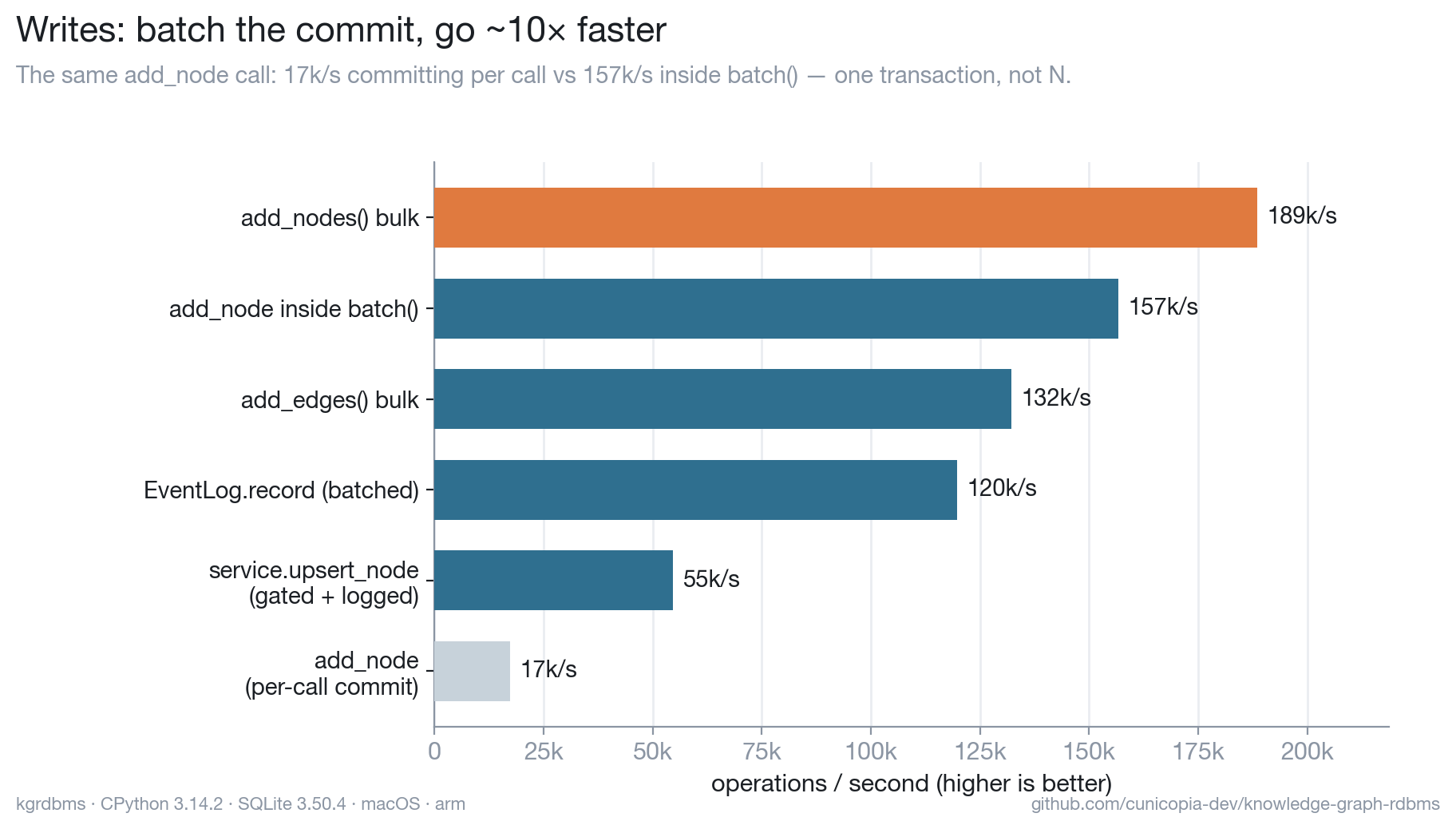
Each single write commits on its own for durability. Wrapping a bulk load in
batch() / add_nodes / add_edges collapses those per-call commits into one
transaction for an ~10× jump — same engine, you just tell it a batch is coming.
The gated + logged path (what the CLI and MCP server use) adds the
invariants+policy check and an event record per write, and still clears tens of
thousands per second.
Reads — fast, with an honest tail
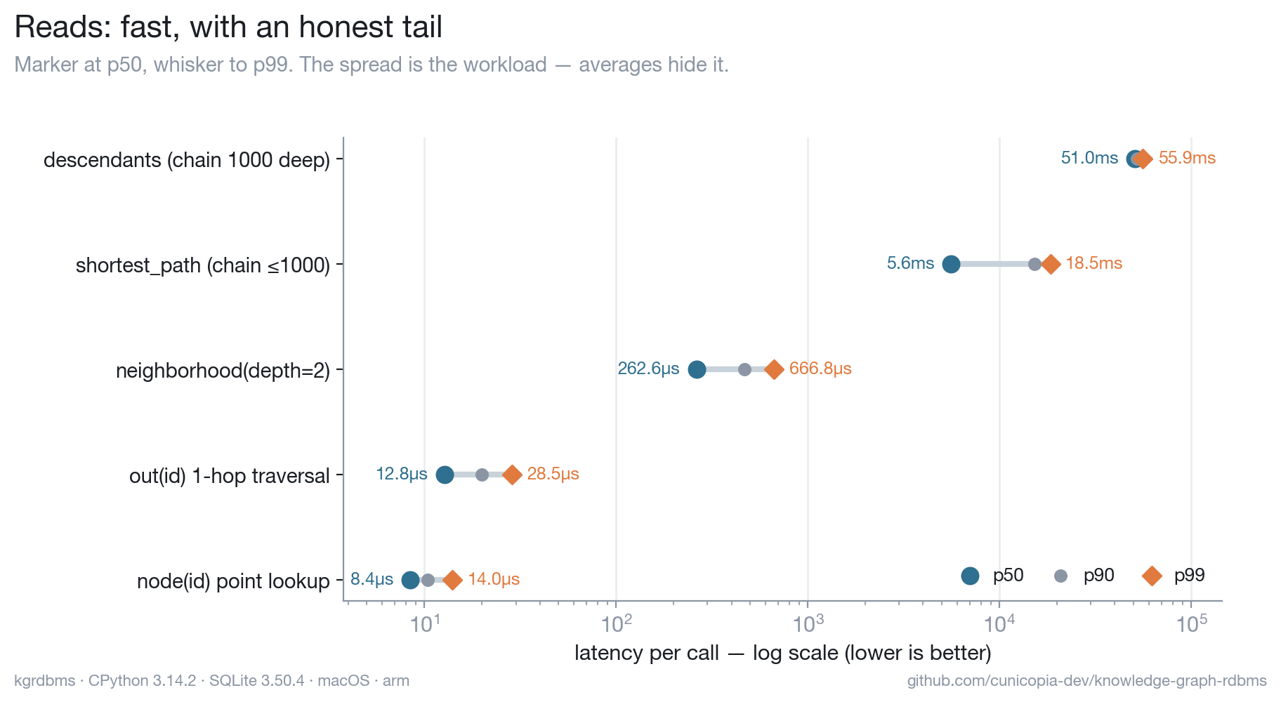
Point lookups land in single-digit microseconds, and multi-node reads hydrate
the whole result set in a constant number of queries (no N+1 fan-out). The chart
plots p50 → p99 on purpose: randomized shortest_path endpoints make some walks
short and some span the whole chain, and an average would bury that tail.
A note on the runtime
kgrdbms is Python, and for performance that's a deliberate non-issue: the same SQLite engine runs under CPython, Node, and Bun, so the gap between them is pure binding overhead — under 2×, and it doesn't even favor one runtime across operations.
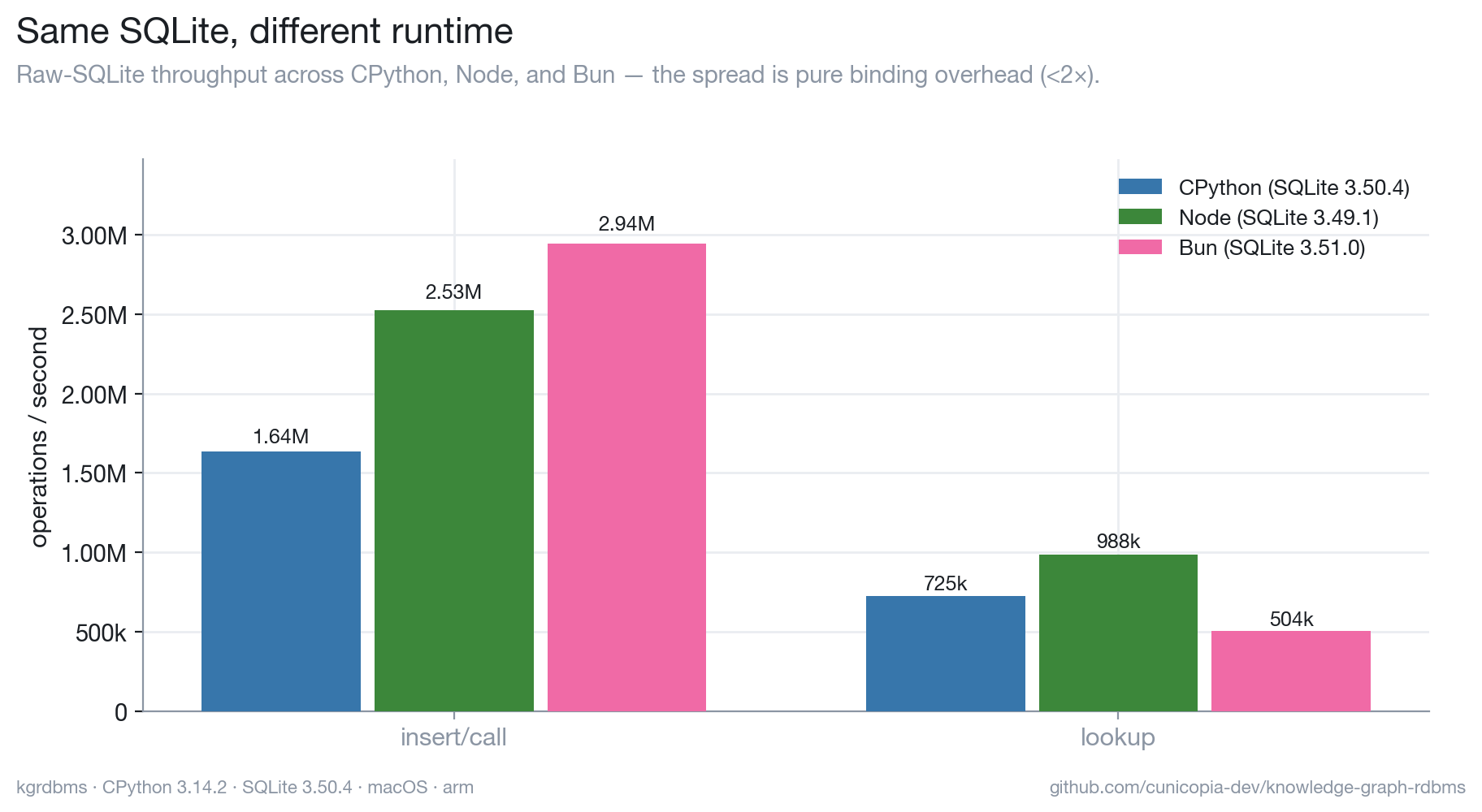
The lever that actually moved the needle was transaction batching (~10×, above),
not the language. Reproduce it with python bench/runtimes/compare.py.
Where the curve bends
We measured it against Neo4j — same graph, same queries, identical methodology
(full harness and reproduction in bench/neo4j/):
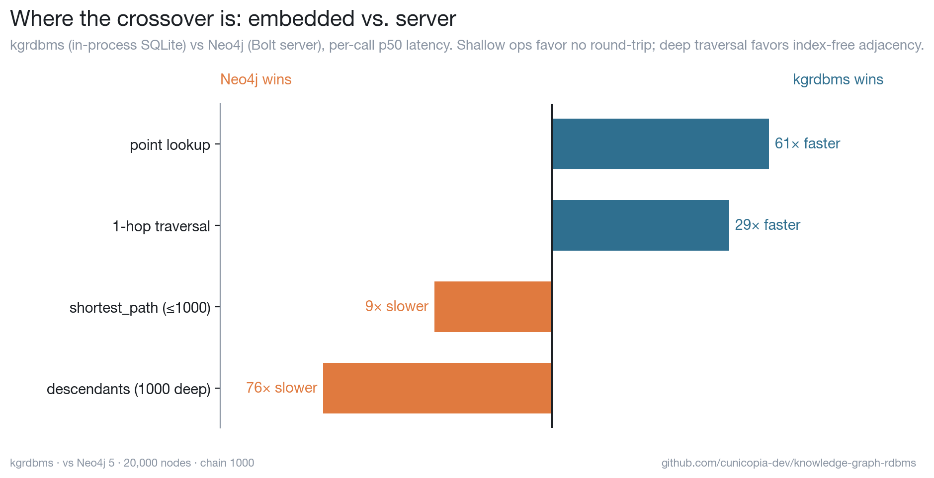
Queries compile to SQL over B-tree indexes, so each traversal hop is an index lookup — wonderfully cheap for point reads and shallow traversals. An in-process lookup here is ~7µs, while the same query to Neo4j pays a Bolt round-trip (~0.4ms) before it even touches data. So for the small, frequent operations that are the bread and butter of agent memory, the embedded graph wins by 30–60×.
A purpose-built engine pulls ahead exactly where the workload — not the row count — turns deep:
- Deep, high-fan-out traversal. Index-free adjacency follows direct pointers between nodes. A 1,000-deep walk costs kgrdbms ~52ms (recursive CTE + row hydration) but ~0.7ms for Neo4j, which pointer-chases under its own round-trip budget — a 76× swing the other way.
- Complex pattern matching. A Cypher planner optimizes multi-pattern queries in ways a fixed traversal API doesn't attempt.
- Concurrent writers and scale-out. Single-file SQLite is one writer at a time; clustered engines aren't.
Rule of thumb: read-heavy and shallow up to low millions of nodes is firmly home turf; deep-traversal or pattern-heavy work is where a dedicated engine earns its complexity. The crossover is workload-shaped, not a single magic number — so we measured ours, and you can measure yours.
SQLite vs the live Postgres engine
Because postgres is a live backend, you can run the same op suite against
both engines and watch the round-trip tax directly
(bench/postgres/). Embedded SQLite wins the small,
frequent ops by 30–60× — a point lookup is in-process, the Postgres one pays a
localhost round-trip. The exception is the one deep traversal that runs as a
single server-side query: the recursive-CTE descendants is where Postgres pulls
ahead (~0.5×), while the per-hop-BFS shortest_path over the same chain is 67×
slower — identical traversal, opposite verdict, decided entirely by how many
times the work crosses the wire. Postgres earns its place on concurrency and
scale, not single-thread latency; the control plane lets you escalate one
ontology to it while the hot, shallow ones stay embedded.
RDF interop: export, SPARQL, RDF-star
The store stays a label property graph. RDF is a boundary format here, not a storage model — there is no triplestore, no OWL, no embedded SPARQL engine. The project adopts exactly one RDF idea, because it is the only one expensive to retrofit: stable identity (CURIE node ids). This is where a CURIE finally expands into a real IRI.
kg rdf export                         # Turtle, to stdout (RDF-star edges)
kg rdf export --format ntriples --out graph.nt
kg rdf import graph.nt                 # back in — gated, logged, replayable
Export is dependency-free. Node ids round-trip as CURIEs, because the prefix binding makes the IRI collapse back to exactly what you stored:
@prefix person: <https://kg.local/person/> .
@prefix kg:     <https://kg.local/vocab#> .

person:ada a kg:Person ;
    kg:name "Ada Lovelace" ;
    prop:born "1815"^^xsd:integer ;
    rel:influences person:grace .

<< person:ada rel:influences person:grace >> prop:since "2020"^^xsd:integer .
That last line is the interesting one. A plain triple has nowhere to hang an
edge's properties; --edge-strategy decides how they cross:
| strategy | edge {since: 2020} becomes | when to use |
|---|---|---|
rdf-star (default) | << :ada :influences :grace >> :since 2020 | star-aware stores (Stardog, Jena 4.3+, Oxigraph) |
reification | an rdf:Statement node carrying s/p/o + each property | rdflib and any RDF 1.1 tool |
lossy | the bare triple; properties dropped (count reported) | you only want topology |
SPARQL? Yes — against the export, in any store. You don't embed a query engine (that would betray the zero-dependency, no-SPARQL design); you emit a graph a real engine can query:
import rdflib
from kgrdbms import rdf

# rdflib is RDF 1.1 — no star — so emit reification for it:
ttl = rdf.export(graph, "turtle", rdf.IriContext(edge_strategy="reification"))
store = rdflib.Graph(); store.parse(data=ttl, format="turtle")
store.query("SELECT ?s ?o WHERE { ?s <https://kg.local/rel/influences> ?o }")
For SPARQL-star over the rdf-star export, hand the Turtle to a star-native
store (Stardog, Jena, Oxigraph, GraphDB). Turtle/foreign-RDF import needs the
optional extra (pip install "knowledge-graph-rdbms[rdf]", which pulls
rdflib); N-Triples import and all export stay dependency-free. Imported RDF
rides the same gated, logged path as every other write, so it is audited and
replayable.
Command reference
| Command | What it does |
|---|---|
kg stats | node/edge counts and db path |
kg schema [--samples] | observed vocabulary: kinds, edge types, labels, keys-per-kind |
kg node add ID --kind K … | create or update a node (gated + logged) |
kg node get ID | fetch a node |
kg node del ID | delete a node (cascades edges) |
kg node set-prop ID KEY VAL | set one property |
kg node add-label ID LABEL | add a label |
kg edge add FROM TO TYPE | add an edge |
kg edge rm FROM TO TYPE | remove an edge |
kg nodes-by-kind KIND | list nodes of a kind |
kg nodes-by-label LABEL | list nodes with a label |
kg out ID [--type T] | outbound edges |
kg in ID [--type T] | inbound edges |
kg path FROM TO | shortest undirected path |
kg neighbors ID [--depth N] | nodes within N hops |
kg descendants ID TYPE | nodes reachable along one edge type |
kg events [-n N] | tail the event log |
kg revert EVENT_ID | undo an event (compensating event) |
kg replay [--upto TS] | rebuild the projection from the log |
kg import FILE | bulk {nodes, edges} import (gated + logged) |
kg rdf export [--format F] | serialize to Turtle/N-Triples (RDF-star) |
kg rdf import FILE | load RDF back in (gated + logged) |
kg ontology list | list registered ontologies (the registry) |
kg ontology create NAME … | register an ontology (--backend, --stance, --shared-identity) |
kg ontology delete NAME [--purge] | deregister an ontology (--purge also deletes its data) |
kg fed schema [--samples] | union vocabulary across ALL ontologies (multithreaded fan-out) |
kg fed stats | node/edge totals across the federation |
kg fed nodes-by-kind KIND / nodes-by-label LABEL | nodes across ontologies, tagged by source |
kg fed node ID | find an id across the federation (identity-aware) |
kg link add FROM_ONT FROM TYPE TO_ONT TO | cross-ontology edge (the backbone) |
kg link same-as A FROM B TO | assert two nodes are the same entity (symmetric) |
kg link of ONT ID | cross-ontology links touching a node |
kg link cluster ONT ID | the transitive SAME_AS identity cluster |
kg prefix add P IRI_BASE | bind a CURIE prefix to an IRI base |
kg prefix expand CURIE / contract IRI | CURIE ↔ IRI via the registry |
kg serve [--transport T] | run the MCP server |
Add --json to any command for machine-readable output. Target a graph with
--ontology NAME (routed through the resolver; default: the default ontology)
or --db PATH (the raw escape hatch onto one exact file, registry bypassed).
Project layout
kgrdbms/
├── graph.py        # the label property graph over SQLite (no internal deps)
├── events.py       # append-only event log: record, compensate, replay
├── policy.py       # configurable mutation policy (permissive by default)
├── invariants.py   # compiled-in invariants, checked before policy (no-op default)
├── service.py      # the shared gated + logged write path
├── resolver.py     # control plane: ontology name → (backend, events, entry) + the index
├── federation.py   # cross-ontology reads: multithreaded fan-out, identity-aware merge
├── backbone.py     # cross-ontology links + prefix/IRI registry (lives in the index graph)
├── backends/       # pluggable engine registry
│   ├── base.py     #   GraphBackend protocol + raising stub skeleton
│   ├── sqlite.py   #   live engine (adapter over Graph)
│   ├── postgres.py #   live engine (psycopg; jsonb + recursive CTEs); [postgres] extra
│   └── neo4j.py    #   stub (deep-traversal escalation)
├── rdf.py          # RDF boundary: Turtle/N-Triples export + import (RDF-star); rdflib only for [rdf] import
├── cli.py          # the `kg` command (stdlib argparse)
└── mcp_server.py   # the MCP server (optional [mcp] extra)
graph.py imports nothing internal — it's a usable, dependency-free LPG on its
own. Everything else layers on top; service.py depends only on the
GraphBackend protocol, never a concrete engine.
Development
git clone <repo> && cd knowledge-graph-rdbms
uv venv && uv pip install -e ".[dev]"
pytest                       # 107 tests
python bench/benchmark.py    # benchmark with p50–p99 (see bench/README.md)
License
MIT.